


![]()
In this article, we will show how data transformations can be an important tool for the proper statistical analysis of data. The association, or correlation, between two variables can be visualised by creating a scatterplot of the data. In certain instances, it may appear that the relationship between the two variables is not linear; in such a case, a linear correlation analysis may still be appropriate. When performing a linear fit of Y against X, for example, an appropriate transformation X’ (of the variable X), Y’ (of the variable Y), or both, can often significantly improve the correlation. A residual plot can reveal whether a data set follows a random pattern, or if a nonlinear relationship can be detected. In such cases, it is often possible to “transform” the raw data to make it more linear. This allows us to use linear correlation techniques more effectively with nonlinear data. Transformations can often significantly improve a fit between X and Y. In other words, if the scatterplot of the raw data (X, Y) looks like that shown in Figure 1 (a), it may be possible to apply a transformation (X’, Y’) to the data so that the scatterplot looks more like that displayed in Figure 1 (b).
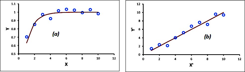
Figure 1 (a) Raw Data and (b) Transformed Data
The main focus of this article will be on the study of special types of transformations to achieve linearity. These are nonlinear transformations that increase the linear relationship between two variables. We will apply the methodology to a real-world problem, where we compare correlations between the online popularity rankings of the most visited websites provided by Ranking.com, and the corresponding MajesticSEO Trust Flow metric.
Data transformation essentially entails the application of a mathematical function to change the measurement scale of a variable that optimizes the linear correlation between the data. The function is applied to each point in a data set — that is, each data point yi is replaced with the transformed value
y’i = f(yi),
Where f is a function. In general, two kinds of transformations can be found in the literature:
- Linear transformation: A linear transformation is one that preserves linear relationships between variables. This implies that the correlation between x and y would remain unchanged after a linear transformation. Some examples of a linear transformation to a variable y would include the multiplication or division of y by a constant (i.e. y’=cy or y’=y/c, where c is a constant), or the addition of a constant to y (y’=y+c).
- Nonlinear transformation: A nonlinear transformation alters (either increases or decreases) the linear relationships between variables and, thus, modifies the correlation between the variables. Examples of a nonlinear transformation of variable y would include taking the logarithm of y (y’=log(y)), or the square root of y (y’=√y).
There are an infinite number of transformations that one could use to achieve linearity for correlation analysis, but it is important to resolve which transformation to apply before proceeding with the statistical calculations. If a cause-and-effect relationship is being tested, the variable that causes the association is called the independent variable and is plotted on the X axis, while the effect is called the dependent variable and is plotted on the Y axis. The specific transformation used can be applied to the dependent and/or independent variables. Some common methods of transforming variables to achieve linearity are described below:
1. If the raw data shows a trend as shown in Figure 2 (a), then it would be appropriate to apply a logarithmic transformation to the dependent variable y as shown in Figure 2 (b). Note that the transformed points lie on a straight line.

Figure 2 (a) Raw Data (b) Transformed Data
This method is known as the Exponential model.
2. If the trend in the data follows the pattern shown in Figure 3 (a), we could take the square root of y to get y’=√y.

Figure 3 (a) Raw Data (b) Transformed Data
This transformation is known as the Quadratic model.
3. A trend in the raw data as shown in Figure 4 (a) would suggest a reciprocal transformation, i.e. y’=1/y.
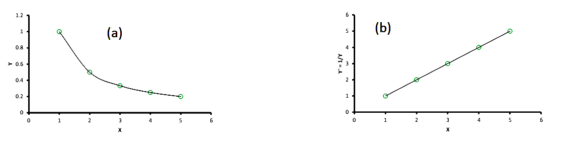
Figure 4 (a) Raw Data (b) Transformed Data
This is the Reciprocal model.
In all of the cases described above, the transformation was applied only to the dependent variable y. In some cases, however, it may be necessary to transform the independent variable x, as described below:
4. If the raw data follows a trend as shown in Figure 5 (a), a logarithmic transformation can be applied to the independent variable x: x’ = log(x).
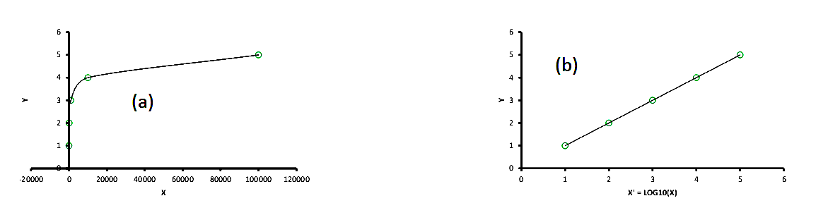
Figure 5 (a) Raw Data (b) Transformed Data
This is known as the Logarithmic model.
Sometimes, transformations may have to be applied to both the dependent and independent variables, as shown in Figure 6 below. In this case, a logarithmic transformation has been applied to both the x and y variables.
5. This method is often referred to as the Power model of data transformation.
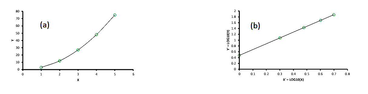
Figure 6 (a) Raw Data (b) Transformed Data
The Box-Cox transformation [1] constitutes another particularly useful family of transformations, which is applied to the independent variable in most cases. The transformation is defined as:
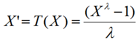 , if λ ≠ 0
T(X) = log(X), if λ = 0
Where X is the variable being transformed and λ is referred to as the transformation parameter. To avoid problems in the case λ = 0, the natural logarithm of X is taken instead of using the above expression.
The Box-Cox linearity plot is a plot of the correlation between the dependent variable Y and the transformed independent variable X for given values of λ, as shown in Figure 7. That is, values of λ are plotted along the horizontal axis, and the values of the correlation between Y and the transformed variable X’ are plotted along the vertical axis of the plot.
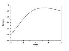
Figure 7: A typical Box-Cox Linearity Plot
The optimal value of λ is then the value of λ corresponding to the maximum correlation (or minimum for negative correlation) on the plot. It is hoped that transforming X can provide a sizeable improvement to the fit. The Box-Cox transformation can also be applied to the Y variable, but this aspect will not be discussed here. One of the advantages of the he Box-Cox linearity plot is that it provides a convenient methodology to determine an appropriate transformation without involving a lot of alternative testing and elimination of failures.
Another method, while not a transformation in the strict sense of the term, is the Spearman Rank Correlation. In a sense, all the Spearman correlation does is transform the data into ranked data, if it has not been transformed already. It’s really just a Pearson correlation applied to ranked or ordinal data. A strong advantage is that the Spearman correlation is less sensitive than the Pearson correlation to strong outliers. When there are no prominent outliers, the Spearman correlation and Pearson correlation give similar values.
We are now in a position to apply the data transformation techniques described above to real-world data. For the purposes of this study, we use the ranking of domains provided by Ranking.com (as determined by the amount of links on other websites on the Internet that point to a particular website or online property), and the proprietary MajesticSEO Trust Flow metric, to establish if there is a correlation between the two, and what transformations are necessary to improve this fit. We used the top 500 ranked sites, and used those sites for which a value of the MajesticSEO Trust Flow was available. After filtering the data, there were 467 sites in the final sample.
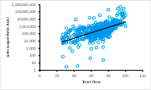
Figure 8: Links (Logarithmic Axis) vs. Trust Flow
Figure 8 shows a plot of the data. The links are plotted on a logarithmic axis, and the black solid line defines the exponential trend line. The Pearson correlation coefficient has a low value of 0.212. The values of the correlation coefficient were calculated using some of the transformations described above to see if any further improvements were possible. The results are summarized in the table shown in Figure 9 below:
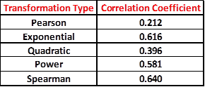
Figure 9: Values for the Correlation Coefficient after Data Transformation
All these values show an improvement over the linear Pearson coefficient. In fact, the Exponential, Power and Spearman transformations display an increase of over 50%, with the Spearman Coefficient having the largest value! Let us see what happens when we apply the Box-Cox transformation to the transformed data described above. We used this link [2] for the Box-Cox transformation to determine if further improvements are possible.
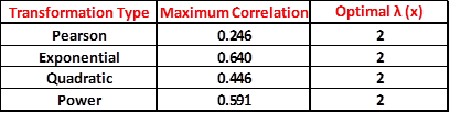
Figure 10: Summary of Box-Cox Linearity Plots
As the table in Figure 10 shows, the maximum correlation that can be achieved increases for all the cases considered. The Spearman Rank Correlation was left out of the computations because it does not make statistical sense to transform ranks. It is seen that the Exponential model can be made to match the Spearman Correlation Coefficient using the Box-Cox data transformation method.
Conclusions:
It has been demonstrated that transforming a data set to enhance linearity can lead to significant improvements in the fit between two variables. This is a multi-step, trial-and-error process. Transformation of data is employed in a manner such that a nonlinear relationship can be transformed to a linear one. These processes also reduce the influence of unusual and extreme variable values, and thus make for more appropriate modelling.
In practice, though, these methods need to be assessed against the data on which they are operated in order to be certain that they result in an increase rather than a decrease in the linearity of the relationship. The efficacy of the transformation method used (exponential model, quadratic model, reciprocal model, etc.) depends on the features of the original data. The only way to determine which method is best is to try each and compare the results obtained (i.e., residual plots, correlation coefficients), as described above. Guidance regarding what data transformation to use, or whether a transform is necessary at all, should come from the particular statistical analysis to be performed, and that too after a rigorous evaluation to determine whether the data closely meets the assumptions of the statistical inference procedure that is to be applied.
Finally, it is worth mentioning that even though a statistical test has been performed on a transformed variable, such as the logarithm, it is in general not good practice to report a summary of the results in transformed units. Instead, the results should be “back-transformed”. This involves doing the opposite of the mathematical function that was used in the data transformation. For example, for the quadratic transformation, back-transforming is achieved by squaring the variable involved. It is very important that a “back transformation” equation is utilized to restore the dependent variable to its original, non-transformed measurement scale.
References
[1] Box, G. E. P. and Cox, D. R. (1964), An Analysis of Transformations, Journal of the Royal Statistical Society, pp. 211-243, discussion pp. 244-252.
[2] Wessa P., (2012), Box-Cox Linearity Plot (v1.0.5) in Free Statistics Software (v1.1.23-r7), Office for Research Development and Education, URL http://www.wessa.net/rwasp_boxcoxlin.wasp/
- Ranking of Top Data Scientists on Twitter using MajesticSEO’s Metrics - August 19, 2014
- Measuring Twitter Profile Quality - August 14, 2014
- PageRank, TrustFlow and the Search Universe - July 7, 2014